Why do we need IoU based loss functions?

A question that may arise when entering the world of object detection is: Why do IoU-based loss functions perform better than L1 loss?

Intuitively, we generally think of object detection as purely a regression problem. So, if we minimize the difference (e.g., L1 or L2 loss) between the predicted and the ground truth bounding boxes, we should get a good model.

This is partially true, but not entirely. Since we evaluate the model using metrics such as mAP, we want to minimize the difference between the predicted and the ground truth bounding box in terms of IoU. In general, the L1 loss does that, but not directly.

Loss landscape

When training a model, we aim to minimize the loss function. We can visualize our model as a “point” in the loss landscape, which we want to move to the global minimum. This movement is entirely dependent on how the gradient behaves in the neighborhood of the current point.

Simply put, the shape of the loss landscape determines how the model learns.

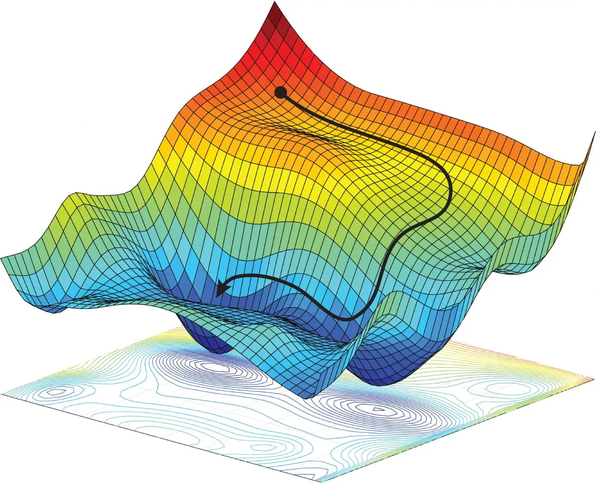
The ball example

Think of our model as a ball in a landscape. We want it to roll to the lowest point.

If the terrain is smooth and sloped (good gradients), the ball rolls naturally to the bottom—just like how optimizers (SGD, Adam) follow the slope. If the terrain is flat, the ball stops moving.

Source

L1 Loss

One of the simplest loss functions used for object detection is the L1 loss. Here, we only minimize the difference between the predicted and ground truth bounding boxes in terms of XY coordinates, not width and height (WH), to allow for visualization on a 2D plane.

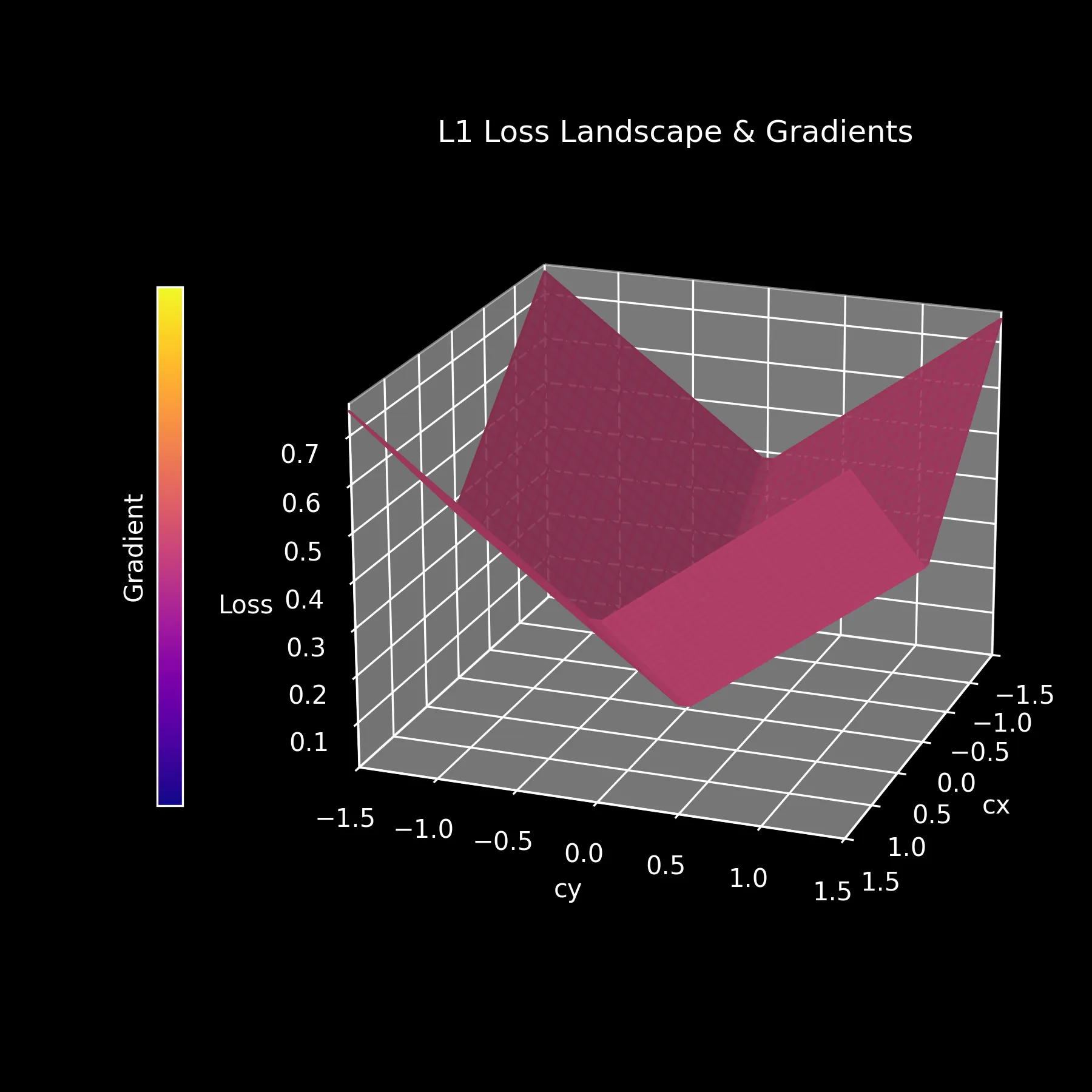
As we can see, the L1 loss landscape is very smooth, with the gradient always pointing toward the minimum. However, the loss is quite “flat”, so the ball will roll down very consistently to find the minimum.

IoU Loss

The IoU loss is defined as $1 - IoU$. It is not widely used, but serves as a good starting point for understanding the problem.

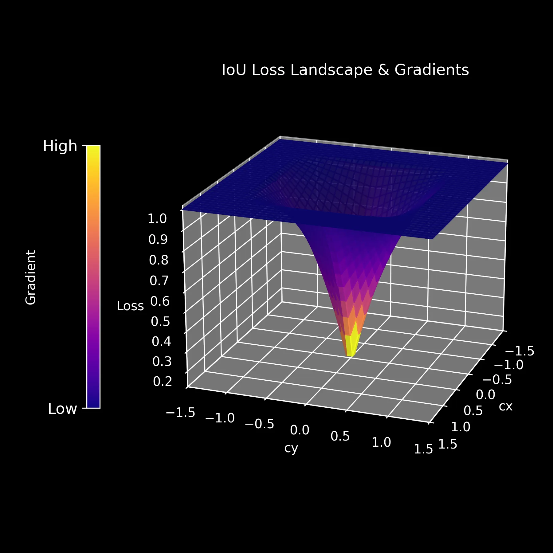
Here’s the problem: The landscape is flat almost everywhere.

If the boxes don’t overlap, IoU is 0, and the loss is 1. Since the value is constant, the gradient is zero.

The model is blind. It knows it’s wrong, but it doesn’t know which way to move to fix it.

The IoU of non-overlapping boxes is 0.

We need a loss function that says:

“Hey, I know you aren’t overlapping the ground truth yet, but go this way and you’ll find it.”

And that’s what GIoU, DIoU, and CIoU loss functions do.

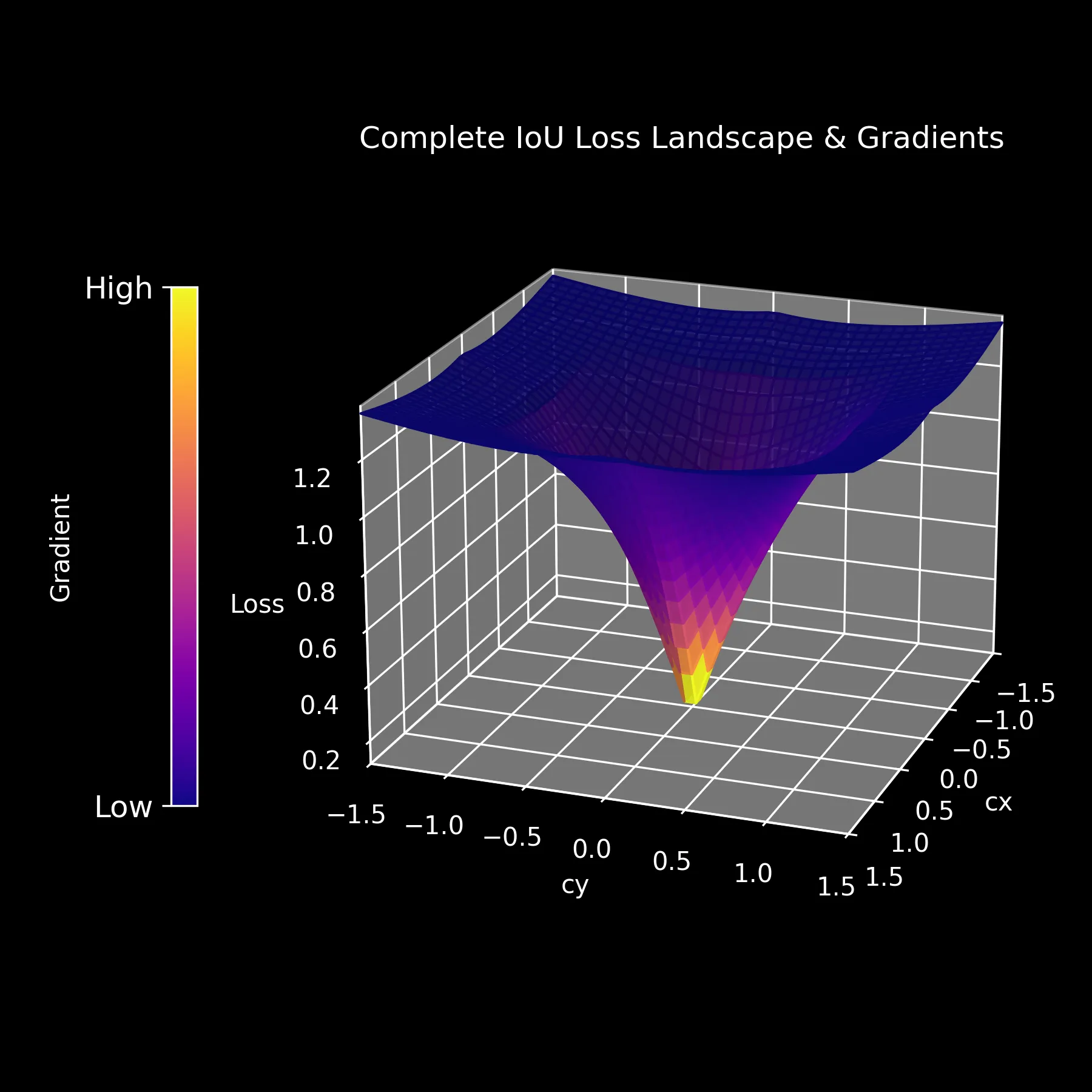
Complete IoU Loss

This was initially proposed in the paper Enhancing Geometric Factors in Model Learning and Inference for Object Detection and Instance Segmentation.

It is defined as a sum of three penalties:

$$L_{CIoU} = \underbrace{1 - IoU}_{\text{Overlap}} + \underbrace{\frac{\rho^2(b, b^{gt})}{c^2}}_{\text{Distance}} + \underbrace{\alpha v}_{\text{Aspect Ratio}}$$

Where:

• Overlap: The standard IoU term.
• Distance: $\rho^2$ is the distance between center points, and $c$ is the diagonal of the enclosing box.
• Aspect Ratio: $\alpha v$ measures if the width/height ratio is consistent.

The CIoU loss landscape is very smooth, and the gradient always points toward the minimum.

Metric Correlation

Theory is nice, but does it work?

Since we evaluate using IoU, we want our loss function to follow it closely. When loss goes down, IoU should go up.

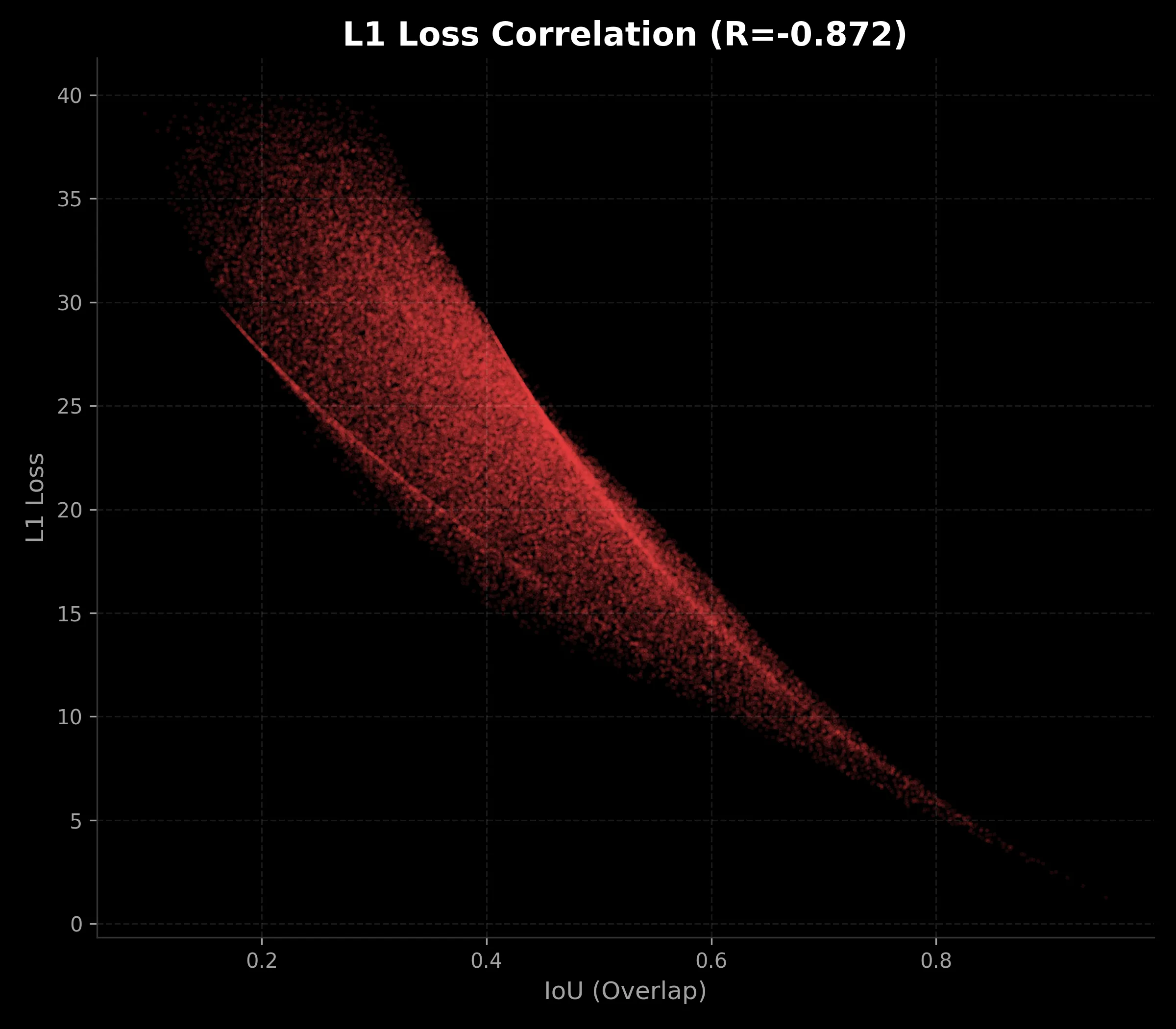
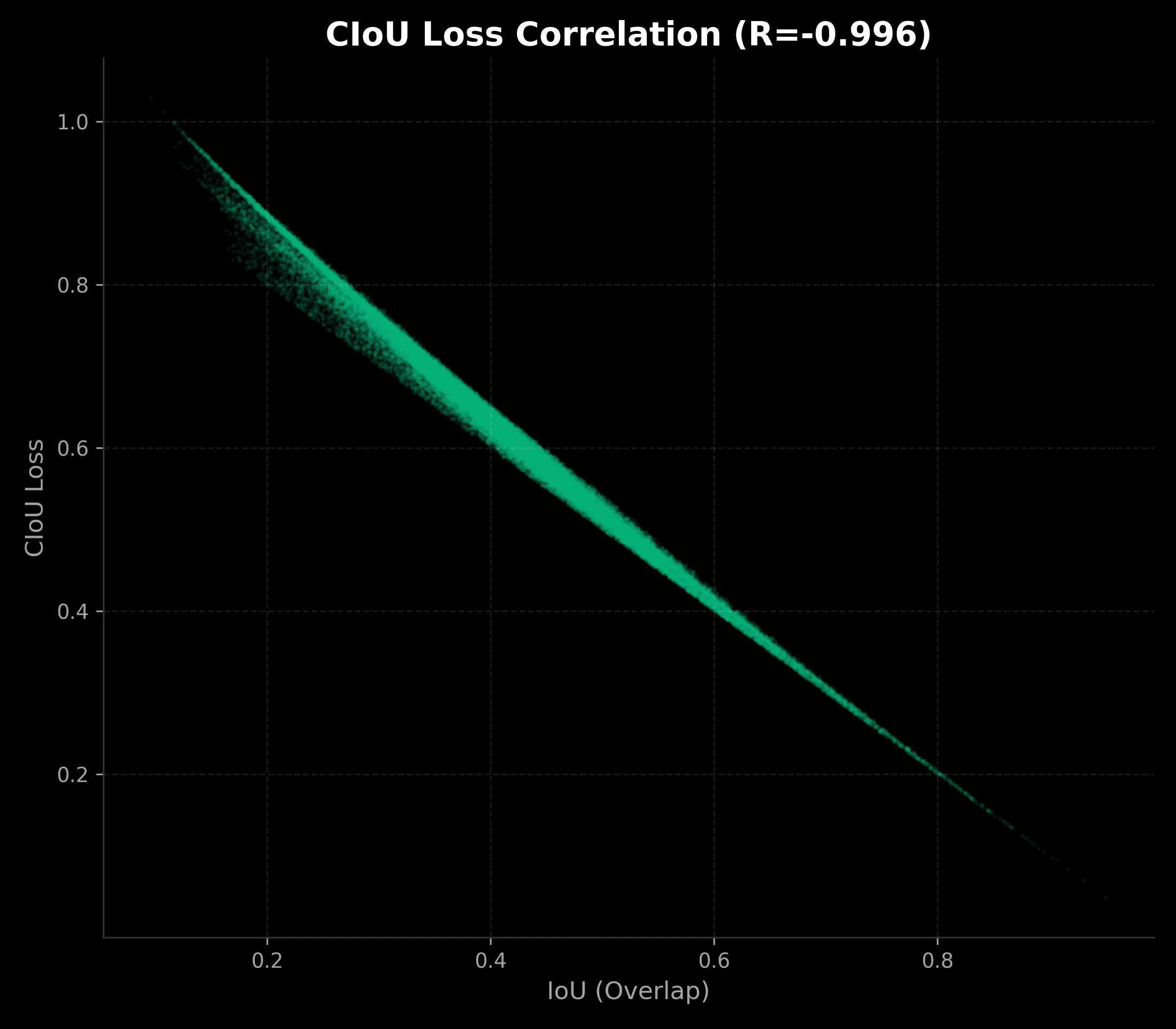
The difference is clear.

• L1 Loss (Left): It’s messy. For the same IoU (e.g., 0.4), the loss can be anywhere from 15 to 30.
• CIoU Loss (Right): It’s a tight curve. A specific loss value almost guarantees a specific IoU.

Conclusion

While L1 loss is simple, it doesn’t align well with how we evaluate detection quality.

IoU-based losses, especially CIoU, bridge that gap. By accounting for overlap, distance, and aspect ratio, they give the model a clear signal on how to improve—even when boxes don’t overlap initially.